Storage and Retrieval

Introduction

On the most fundamental level, a database needs to do two things: when you give it some data, it should store the data, and when you ask it again later, it should give the data back to you.

Why should you, as an application developer, care how the database handles storage and retrieval internally? You're probably not going to implement your own storage engine from scratch, but you do need to select a storage engine that is appropriate for your application, from the many that are available. In order to tune a storage engine to perform well on your kind of workload, you need to have a rough idea of what the storage engine is doing under the hood.

First, we'll start this chapter by talking about storage engines that are used in the kinds of databases that you're probably familiar with: traditional relational databases, and also most so-called NoSQL databases. We will examine two families of storage engines: log-structured storage engines, and page-oriented storage engines such as B-trees.

Data Structures That Power Your Database

An index is an additional structure that is derived from the primary data. Many databases allow you to add and remove indexes, and this doesn't affect the contents of the database; it only affects the performance of queries. Maintaining additional structures incurs overhead, especially on writes. For writes, it's hard to beat the performance of simply appending to a file, because that's the simplest possible write operation. Any kind of index usually slows down writes, because the index also needs to be updated every time data is written.

B-Trees

The most widely used indexing structure is quite different: the B-tree.

B-trees have stood the test of time very well. They remain the standard index implementation in almost all relational databases, and many nonrelational databases use them too.

B-trees keep key-value pairs sorted by key, which allows efficient key-value lookups and range queries. But that's where the similarity ends: B-trees have a very different design philosophy.

B-trees break the database down into fixed-size blocks or pages, traditionally 4 KB in size (sometimes bigger), and read or write one page at a time. This design corresponds more closely to the underlying hardware, as disks are also arranged in fixed-size blocks.

Each page can be identified using an address or location, which allows one page to refer to another—similar to a pointer, but on disk instead of in memory. We can use these page references to construct a tree of pages, as illustrated in the image below.

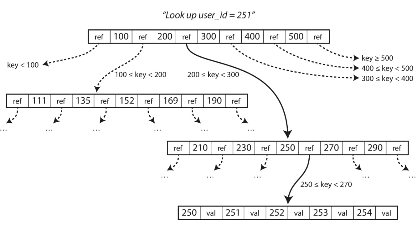Looking up a key using a B-tree index

One page is designated as the root of the B-tree; whenever you want to look up a key in the index, you start here. The page contains several keys and references to child pages. Each child is responsible for a continuous range of keys, and the keys between the references indicate where the boundaries between those ranges lie.

In the example image above, we are looking for the key 251, so we know that we need to follow the page reference between the boundaries 200 and 300. That takes us to a similar-looking page that further breaks down the 200-300 range into subranges. Eventually we get down to a page containing individual keys (a leaf page), which either contains the value for each key inline or contains references to the pages where the values can be found.

If you want to update the value for an existing key in a B-tree, you search for the leaf page containing that key, change the value in that page, and write the page back to disk (any references to that page remain valid). If you want to add a new key, you need to find the page whose range encompasses the new key and add it to that page. If there isn't enough free space in the page to accommodate the new key, it is split into two half-full pages, and the parent page is updated to account for the new subdivision of key ranges.

This algorithm ensures that the tree remains balanced: a B-tree with n keys always has a depth of O(log n). Most databases can fit into a B-tree that is three or four levels deep, so you don't need to follow many page references to find the page you are looking for. (A four-level tree of 4 KB pages with a branching factor of 500 can store up to 256 TB.)

Making B-trees reliable

Some operations require several different pages to be overwritten. For example, if you split a page because an insertion caused it to be overfull, you need to write the two pages that were split, and also overwrite their parent page to update the references to the two child pages. This is a dangerous operation, because if the database crashes after only some of the pages have been written, you end up with a corrupted index (e.g., there may be an orphan page that is not a child of any parent).

In order to make the database resilient to crashes, it is common for B-tree implementations to include an additional data structure on disk: a write-ahead log (WAL, also known as a redo log). This is an append-only file to which every B-tree modification must be written before it can be applied to the pages of the tree itself. When the database comes back up after a crash, this log is used to restore the B-tree back to a consistent state.

An advantage of B-trees is that each key exists in exactly one place in the index. This aspect makes B-trees attractive in databases that want to offer strong transactional semantics: in many relational databases, transaction isolation is implemented using locks on ranges of keys, and in a B-tree index, those locks can be directly attached to the tree.

Other Indexing Structures

It is also very common to have secondary indexes. In relational databases, you can create several secondary indexes on the same table using the CREATE INDEX command, and they are often crucial for performing joins efficiently.

Multi-column indexes

The indexes discussed so far only map a single key to a value. That is not sufficient if we need to query multiple columns of a table (or multiple fields in a document) simultaneously.

The most common type of multi-column index is called a concatenated index, which simply combines several fields into one key by appending one column to another (the index definition specifies in which order the fields are concatenated). This is like an old-fashioned paper phone book, which provides an index from (lastname, firstname) to phone number. Due to the sort order, the index can be used to find all the people with a particular last name, or all the people with a particular lastname-firstname combination. However, the index is useless if you want to find all the people with a particular first name.

Full-text search and fuzzy indexes

All the indexes discussed so far assume that you have exact data and allow you to query for exact values of a key, or a range of values of a key with a sort order. What they don’t allow you to do is search for similar keys, such as misspelled words. Such fuzzy querying requires different techniques.

Full-text search engines commonly allow a search for one word to be expanded to include synonyms of the word, to ignore grammatical variations of words, and to search for occurrences of words near each other in the same document, and support various other features that depend on linguistic analysis of the text.

Keeping everything in memory

Many datasets are simply not that big, so it's quite feasible to keep them entirely in memory, potentially distributed across several machines. This has led to the development of in-memory databases.

When an in-memory database is restarted, it needs to reload its state, either from disk or over the network from a replica (unless special hardware is used). Despite writing to disk, it's still an in-memory database, because the disk is merely used as an append-only log for durability, and reads are served entirely from memory. Writing to disk also has operational advantages: files on disk can easily be backed up, inspected, and analyzed by external utilities.

Counterintuitively, the performance advantage of in-memory databases is not due to the fact that they don't need to read from disk. Even a disk-based storage engine may never need to read from disk if you have enough memory, because the operating system caches recently used disk blocks in memory anyway. Rather, they can be faster because they can avoid the overheads of encoding in-memory data structures in a form that can be written to disk.

Besides performance, another interesting area for in-memory databases is providing data models that are difficult to implement with disk-based indexes. For example, Redis offers a database-like interface to various data structures such as priority queues and sets. Because it keeps all data in memory, its implementation is comparatively simple.

Transaction Processing or Analytics?

In the early days of business data processing, a write to the database typically corresponded to a commercial transaction taking place: making a sale, placing an order with a supplier, paying an employee's salary, etc. As databases expanded into areas that didn't involve money changing hands, the term transaction nevertheless stuck, referring to a group of reads and writes that form a logical unit.

An application typically looks up a small number of records by some key, using an index. Records are inserted or updated based on the user's input. Because these applications are interactive, the access pattern became known as online transaction processing (OLTP).

However, databases also started being increasingly used for data analytics, which has very different access patterns. Usually an analytic query needs to scan over a huge number of records, only reading a few columns per record, and calculates aggregate statistics (such as count, sum, or average) rather than returning the raw data to the user. For example, if your data is a table of sales transactions, then analytic queries might be:

• What was the total revenue of each of our stores in January?

• How many more bananas than usual did we sell during our latest promotion?

In order to differentiate this pattern of using databases from transaction processing, it has been called online analytic processing (OLAP).

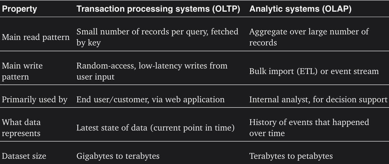Comparing characteristics of transaction processing versus analytic systems

Data Warehousing

An enterprise may have dozens of different transaction processing systems: systems powering the customer-facing website, controlling point of sale (checkout) systems in physical stores, tracking inventory in warehouses, planning routes for vehicles, managing suppliers, administering employees, etc. Each of these systems is complex and needs a team of people to maintain it, so the systems end up operating mostly autonomously from each other.

These OLTP systems are usually expected to be highly available and to process transactions with low latency, since they are often critical to the operation of the business.

A data warehouse, by contrast, is a separate database that analysts can query to their hearts' content, without affecting OLTP operations. The data warehouse contains a read-only copy of the data in all the various OLTP systems in the company. Data is extracted from OLTP databases (using either a periodic data dump or a continuous stream of updates), transformed into an analysis-friendly schema, cleaned up, and then loaded into the data warehouse. This process of getting data into the warehouse is known as Extract-Transform-Load (ETL). This is illustrated in the image below.

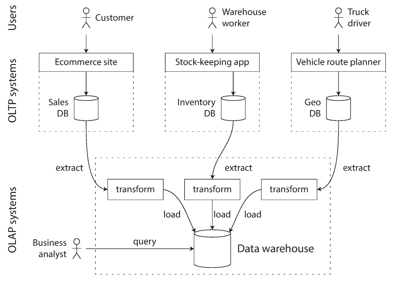Simplified outline of ETL into a data warehouse

A big advantage of using a separate data warehouse, rather than querying OLTP systems directly for analytics, is that the data warehouse can be optimized for analytic access patterns.

The divergence between OLTP and data warehouses

On the surface, a data warehouse and a relational OLTP database look similar, because they both have a SQL query interface. However, the internals of the systems can look quite different, because they are optimized for very different query patterns. Many database vendors now focus on supporting either transaction processing or analytics workloads, but not both.

Column-Oriented Storage

Before we can understand column-oriented storage, we need to understand what a fact table is. A fact table is a table where each row represents an event that occurred at a particular time.

If you have trillions of rows and petabytes of data in your fact tables, storing and querying them efficiently becomes a challenging problem. Although fact tables are often over 100 columns wide, a typical data warehouse query only accesses 4 or 5 of them at one time (SELECT * queries are rarely needed for analytics).

In most OLTP databases, storage is laid out in a row-oriented fashion: all the values from one row of a table are stored next to each other. Document databases are similar: an entire document is typically stored as one contiguous sequence of bytes.

The idea behind column-oriented storage is simple: don't store all the values from one row together, but store all the values from each column together instead. If each column is stored in a separate file, a query only needs to read and parse those columns that are used in that query, which can save a lot of work

Column Compression

Besides only loading those columns from disk that are required for a query, we can further reduce the demands on disk throughput by compressing data. Fortunately, column-oriented storage often lends itself very well to compression.

Summary

In this chapter we tried to get to the bottom of how databases handle storage and retrieval. What happens when you store data in a database, and what does the database do when you query for the data again later?

On a high level, we saw that storage engines fall into two broad categories: those optimized for transaction processing (OLTP) and those optimized for analytics (OLAP). There are big differences between the access patterns in those use cases:

• OLTP systems are typically user-facing, which means that they may see a huge volume of requests. In order to handle the load, applications usually only touch a small number of records in each query. The application requests records using some kind of key, and the storage engine uses an index to find the data for the requested key. Disk seek time is often the bottleneck here.

• Data warehouses and similar analytic systems are less well known, because they are primarily used by business analysts, not by end users. They handle a much lower volume of queries than OLTP systems, but each query is typically very demanding, requiring many millions of records to be scanned in a short time. Disk bandwidth (not seek time) is often the bottleneck here, and column-oriented storage is an increasingly popular solution for this kind of workload.

Finishing off the OLTP side, we did a brief tour through some more complicated indexing structures, and databases that are optimized for keeping all data in memory.

We then took a detour from the internals of storage engines to look at the high-level architecture of a typical data warehouse. This background illustrated why analytic workloads are so different from OLTP: when your queries require sequentially scanning across a large number of rows, indexes are much less relevant. Instead it becomes important to encode data very compactly, to minimize the amount of data that the query needs to read from disk. We discussed how column-oriented storage helps achieve this goal.